Malcolm Coles

The formulae from my talk on creating your own rank tracker using Google Search Console, Looker Studio and Google Sheets.

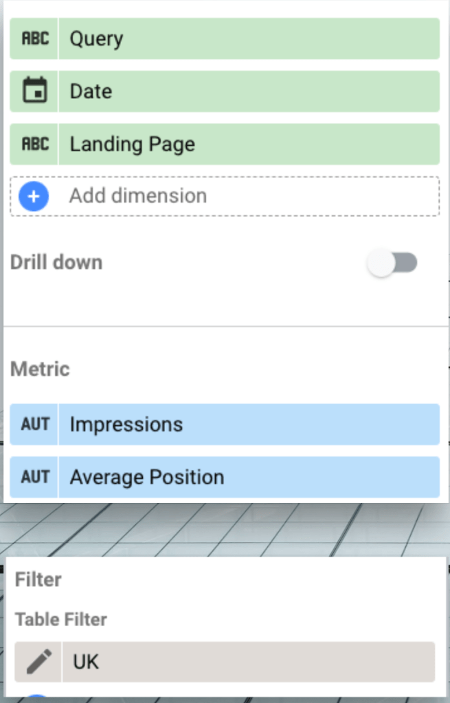
Get the data from GSC, into looker studio and then export to sheets.

Sort out the date

=arrayformula(month(B2:B))

=arrayformula(DAY(B2:B))

Then combine month and date with EG =date(2023,D2,E2) (this is all to cope with September coming through as Sept and sheets not recognising it) and applying a date format

Combine page and query

=arrayformula(A2:A&" : "&C2:C)

Work out how many times each page query combo appears

={unique(I2:I),
ArrayFormula(sumif(I2:I,unique(I2:I),G2:G))}

Add that impressions number to each row that’s showing page, query and date

=arrayformula(vlookup(I2:I,K$2:L,2, false))

You should end up with these columns:

Make a pivot table (you need columns F to J in my example)

Add some extra data

=counta(C3:AG3)

=AH3/AI3

Get the main columns and split them

=query('Pivot Table 1'!A3:AJ,"select B,A,AJ")

=arrayformula(split(D2:D," : ",false))

Get the rankings columns, replace blanks with 100

=min('Pivot Table 1'!C3,100)

Make the graphs

=SPARKLINE(F2:AF2,
{"empty","ignore";"charttype","line";
"ymin",20;"ymax",0;"color","blue";"linewidth",2})